Article contents
- Evidence and scope
- Illustration
- Process
- A fitted line describes the observed window
- Fit only observations preceding the detection bar
- A return inside the channel can succeed or fail
- Frozen coefficients can still imply a moving center
- Residual diagnostics are not a profitability certificate
- Volume can filter events without rewriting the channel
- Chronological tests and useful controls
- Common pitfalls
- Practical checklist
- Frequently asked questions
- Research sources
Evidence and scope
Fidelity explains a regression indicator, while statsmodels and NIST support fitting and diagnostics. None establishes profitability for the proposed channel-reclaim strategy.
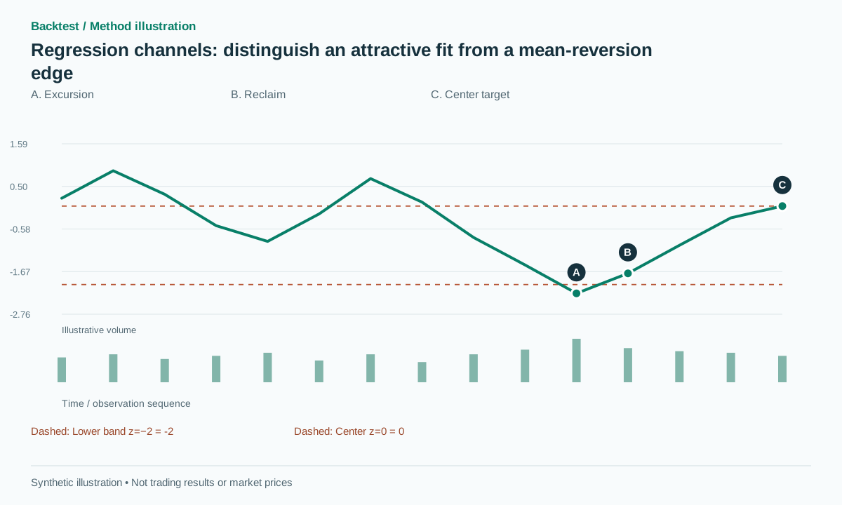 Open full-size illustration
Practical workflow
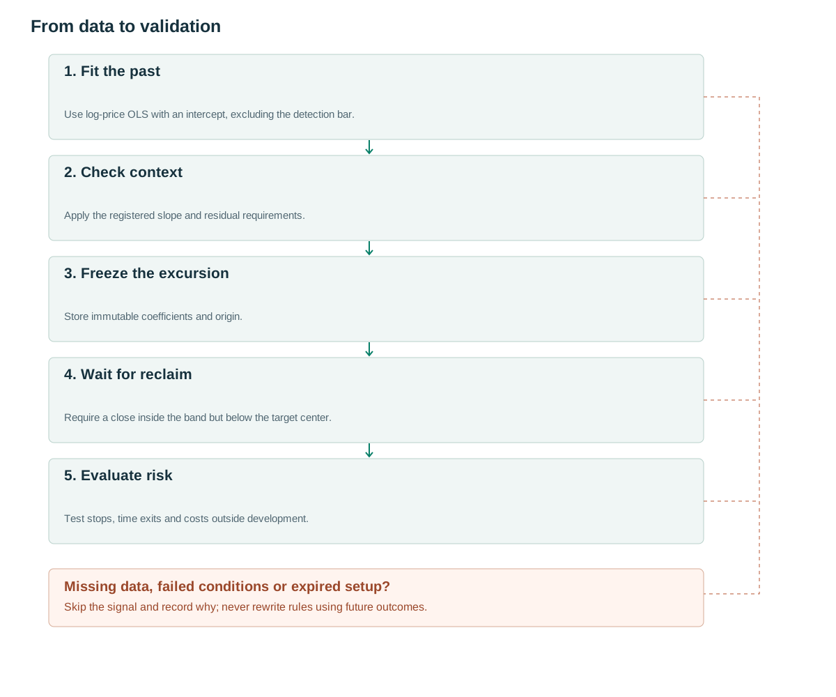
- Fit the pastUse log-price OLS with an intercept, excluding the detection bar.
- Check contextApply the registered slope and residual requirements.
- Freeze the excursionStore immutable coefficients and origin.
- Wait for reclaimRequire a close inside the band but below the target center.
- Evaluate riskTest stops, time exits and costs outside development.
A fitted line describes the observed window
Fidelity describes its Linear Regression Indicator through the endpoint of a fitted line over N periods [1]. This article extends that descriptive idea with residual bands. A sloping center means that being far below the line does not automatically imply fundamental cheapness or an imminent rise.
Separate two questions: how well a straight line explains the past window, and whether today's deviation predicts a subsequent return. R² answers the first. A steady decline can have high R² while buying below its fitted line repeatedly loses money.
A channel can be used for mean reversion or trend continuation, but these are competing hypotheses. The baseline below waits for a downside excursion and a return inside the frozen lower band. It does not switch to momentum when a historical mean-reversion trade fails.
Fit only observations preceding the detection bar
For j=0…N−1, set y[j]=log(C[j]) and fit y=a+bj by ordinary least squares. Residuals are e[j]=y[j]−a−bj and s=sqrt(sum(e²)/(N−2)). At h steps beyond the fitted window, m(h)=a+b(N−1+h), with price bands exp(m(h)±ks). Proposed settings are N=60, k=2; reject nonpositive prices and near-zero s.
statsmodels OLS does not automatically add an intercept to a supplied design matrix [2], so include a constant column. Fit through t−1 and evaluate close t at h=1. Including t would let the shock move both the center and the width being used to judge that same shock.
The proposed range-context filter abs(b)×(N−1)/s≤1 compares fitted drift with residual scale. It is a screening rule, not a stationarity test. Save a, b, s, the origin index and the fitted input window when an excursion creates a candidate. Never refit that active candidate.
Expiry must take precedence over triggering. The pseudocode makes that ordering explicit and initializes previous_z when the excursion is first detected. Missing data, nonfinite fit results and zero residual scale disable the candidate rather than allowing division by zero or an artificial extreme z-score.
if no_candidate:
    if invalid_or_nonpositive(close[t-N:t+1]): return
    a,b,s = fit_log_ols(close[t-N:t], with_intercept=True)
    if not finite(a,b,s) or s <= min_residual_scale: return
    regime_ok = abs(b)*(N-1)/s <= 1.0
    z = (log(C[t])-(a+b*N))/s
    if regime_ok and z < -2:
        freeze_candidate(a,b,s,origin=t-N,expiry=t+10,
                         previous_z=z,excursion_low=L[t])
else:
    if t > candidate.expiry:
        expire(); return
    j = t-candidate.origin
    z = (log(C[t])-(candidate.a+candidate.b*j))/candidate.s
    update_excursion_low(L[t])
    if candidate.previous_z < -2 and -2 <= z < 0:
        emit_long(t)
    candidate.previous_z = z
# Never refit an active candidate or backfill historical channels.
A return inside the channel can succeed or fail
Synthetic example: the fitted center is approximately 100, slope0 and log residual scale s=0.01. The two-sigma lower band is approximately 98.02 and upper band102.02. Price 97.8 is outside the lower band; a subsequent close 98.3 re-enters. Entry 98.4, stop 97.5 and target 100 imply risk 0.9 and potential reward 1.6, or approximately 1.78R before costs.
The successful synthetic path reaches 100 first. In the failure path, new information drives price to 96 and then94. The position must stop at a feasible price near97.5 or worse if it gaps. A good historical fit cannot prevent a change in the price-generating environment.
Do not widen sigma after the decline and declare that the earlier stop was never truly broken. That would change the decision snapshot using the outcome. Model updates for future candidates must not alter the accounting of an existing trade.
Another path jumps directly from 97.8 to 101. Although it has returned inside the band, the baseline requires z<0 and therefore does not buy above its center target. This rule is fixed in advance rather than added after seeing a poor reward-to-risk gap.
Frozen coefficients can still imply a moving center
Freezing a and b does not make the projected center horizontal. It continues along the original slope as the time index advances. At the signal, freeze a target equal to the center projected for the expected entry time and a stop below the entire excursion low minus a buffer.
The proposed position has a ten-bar time exit if neither target nor stop is reached. Candidate expiry and position time exit are different clocks: one limits waiting for a reclaim, the other limits holding after entry. Store both to avoid extending a candidate accidentally when a trade opens.
If execution is delayed beyond the expected entry time, define whether the frozen target stays unchanged or is canceled before submission under an economics rule. Do not move the target after a fill merely to keep potential reward attractive.
Compare next-open and executable-quote assumptions around fast moves. A historical line crossing is not a guaranteed fill at the line. If the target is a resting limit, model its activation, quantity and potential nonfill rather than automatically crediting the center price whenever a later bar spans it.
Residual diagnostics are not a profitability certificate
NIST discusses classical residual assumptions such as independence and stable variance [3]. Financial prices can violate them. Consequently,±2s is not automatically a 95% forecast interval for the next price, and a conventional OLS slope p-value is not evidence of a tradable edge.
Inspect residual autocorrelation, tail behavior and stability of s across windows. Persistent residuals on one side may indicate that the strategy is fading a new trend. These diagnostics should explain model behavior without being used to select only favorable historical episodes.
A practical comparison keeps frozen snapshots for every candidate and plots price movement relative to those snapshots. If apparent reversion occurs only because a repeatedly refitted center moves toward price, the effect is model adaptation rather than price returning to its original reference.
R², standard error and z-score serve different purposes. R² describes fit, standard error summarizes in-window residual scale, and z-score expresses a current deviation under that frozen scale. None should be relabeled as a probability of the next trade winning.
Volume can filter events without rewriting the channel
One proposed hypothesis avoids fading unusually high RVOL because it may accompany repricing. A competing hypothesis looks for high excursion activity followed by quieter reclaim activity. Choose and register a feature before examining trade outcomes instead of applying both stories whenever convenient.
Use a same-time baseline, record spreads and timestamped news if available, and prevent completed-excursion volume from informing a decision before the excursion ends. At reclaim confirmation, the observed excursion can be summarized, but the feature's available_at must reflect its latest input.
Changing OLS to volume-weighted regression changes the model itself. Evaluate it as a distinct version against the unweighted baseline. Otherwise, a reported benefit from volume may combine a changed center, a changed residual scale and a changed entry filter without identifying which component matters.
Chronological tests and useful controls
Compare the regression channel with a flat Bollinger-style mean and a no-slope z-score baseline under equivalent entry, exit and cost policies. Select N, k and the context filter on development data, then preserve a final unseen test. Purge overlapping trade-label intervals when a split would otherwise share the same excursion outcome.
Implementation fixtures should verify the intercept, the t−1 window end, log scaling, degrees of freedom, zero s, missing observations and prefix invariance. Test an expired candidate that re-enters on the next bar: it must remain expired rather than emit a late signal.
Report net return, tail loss, no-trade time and performance by previously defined regime. Stress fills and gaps. If profitability depends on crediting an exact center fill inside an ambiguous gap bar, the execution model needs correction before economic conclusions are drawn.
A higher-order polynomial may fit history more closely while adding unstable extrapolation and more research choices. The linear baseline is valuable because its coefficients, projection and failure cases can be audited directly.
Common pitfalls
Refitting historical channels
The current line rewrites earlier signals and makes the chart appear consistently accurate.
Turning R² into win rate
In-sample explanatory fit is not the same as predictive trading performance.
Fading a regime change
The old channel can lose relevance when new information reprices the instrument.
Checklist before using this method
Check each item after verifying it on your data. Progress is saved in this browser; it does not certify a profitable strategy.
Frequently asked questions
Is regression always better than Bollinger Bands?
No. It adds a slope and model choices. Compare under matched trading and execution rules to isolate their value.
Can a polynomial improve the fit?
It can be researched, but adds degrees of freedom and extrapolation risk. A closer historical fit alone does not establish a better strategy.
Research sources
Each source supports the definition or evidence described beside it. The pseudocode, synthetic examples and proposed parameters require separate validation.
- Linear Regression IndicatorFidelity. Read the regression indicator's endpoint definition. Checked: .
- statsmodels OLSstatsmodels. Read OLS intercept, missing-data and fit behavior. Checked: .
- Are the model residuals well-behaved?NIST/SEMATECH. Read classical residual assumptions; these are not conclusions about market predictability. Checked: .
Related methods
Risk note
This content supports education and research design, not financial advice. Backtest is historical simulation, does not guarantee future performance and does not place real trades. Methods in this library are not automatically features available in the app. See methodology and learning center.
Validate rules before risking real capital
Check app support, data and individual simulated trades; advanced detectors may require a separate implementation.
Download Backtest on the App Store